Observation and modelling of various hydrological processes in a small watershed in the Upper Ganga basin
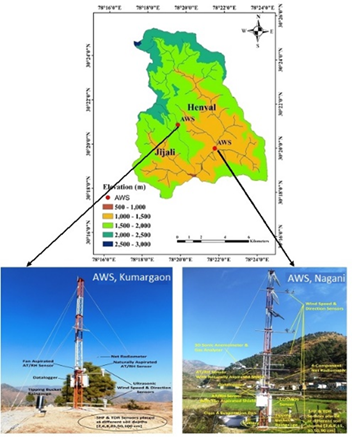
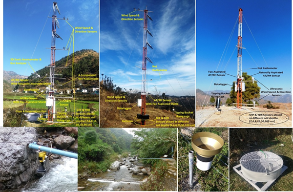
Understanding the interaction among atmospheric, land surface and hydrological processes and their seasonal variation is key to understand the response of climate change. For this purpose, two small hilly watersheds (Henval and Jijali) located in Tehri Garhwal district of Uttarakhand State in upper Ganga basin have been selected as shown in Figure – 1. Jijali watershed is forested while the Henval watershed is agriculture-dominated and these two are good representative of lesser Himalayan hilly temperate climatic conditions. Extensive field monitoring of various hydro-meteorological and soil variables has been done in these watersheds at various elevations as shown in Figure – 2. Using 3 AWS, meteorological profile system is mounted within which air temperature, relative humidity; wind speed, wind direc¬tion, atmospheric pressure, soil moisture, soil heat flux and net radiation are measured simultaneously. Sensors are placed at 15 cm, 30 cm, 50 cm and 90 cm depths in soil to monitor different variables. Continuous gauging is being done by using broad crested rectangular and trapezoidal constructed weirs just upstream of their outlets. Staff gauges have also been installed to monitor the water levels. An automatic water level recorder (AWLR) is installed on the Henval stream just upstream of the weir. Ordinary rain gauges (10 Nos.) have been installed at appropriate locations (in different elevation bands) of watersheds. A pan evaporimeter has been installed near Henval AWS. Local peoples have been trained for daily monitoring of Pan and ORG’s.
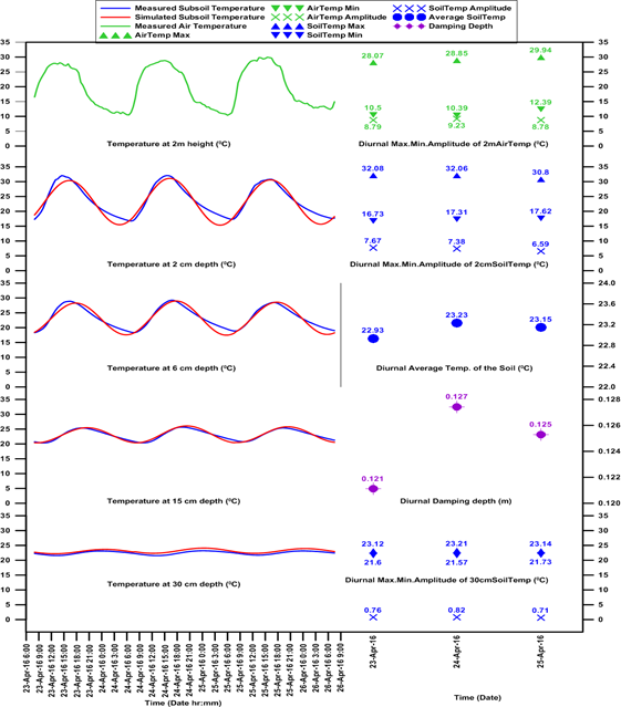
The experimental data generated in the study have been used to carry out various analysis and modelling exercises such as subsoil temperature analysis, simulation of apparent thermal diffusivity, estimation of roughness length for momentum (Z0m), modelling of water balance components, assessment of potential evapotranspiration, soil erosion and sediment yield modeling etc. Using the daily maximum and minimum temperatures at two depths (2 & 30 cm) in a homogeneous soil profile as well as 2-m above the ground and average temperature of the soil profile, a sinusoidal model has been proposed which can predict the soil temperature at any time and depth. The results are shown in Figure – 3.
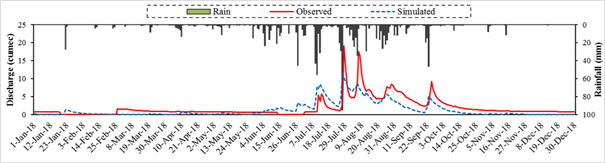
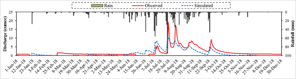
Roughness length for momentum (Z0m) is defined as the height above the surface at which the mean logarithmic wind profile reaches zero. It is affected by aerodynamic and thermodynamic factors and rough elements, including wind speed, wind direction, terrain, atmospheric stratification, and LAI. In this study, variation of roughness length (Z0) and wind speed in various seasons and months of a year have been observed. One of the major drivers of large seasonal variations in Z0is the distinct seasonal pattern of the leaf area index (LAI) which increases from a minimum at the beginning of the growing season (early May) to a maximum in late June and starts to decrease in the middle of September. At the beginning of the growing season, the LAI is relatively low and new leaves are very soft. The resistance to flow on the canopy surface is small, which results in small Z0. With increase in the LAI and ag-ing of the leaves, the resis¬tance and consequently roughness length increases. Further with crop maturity, the LAI starts to decrease and consequently Z0 starts to decrease. During the non-growing season, low vegetation/canopy density results in lower Z0. Water balance is defined as the numerical calculation accounting for the inputs to, outputs from, and changes in the volume of water in the various components (e.g. reservoir, river, aquifer) of the hydrological cycle, within a specified hydrological unit (e.g. river basin) and during a specified time unit (e.g. month/year), occurring both naturally and as a result of the human-induced water abstractions and returns. In this study, water balance components of the watershed have been estimated by using the Thornthwaite method and SWAT model. Thornthwaite model requires the mean monthly temperature and monthly total precipitation while the SWAT model requires spatial data like DEM, land use map, soil map and meteorological data. The results of SWAT model durng calibration and validations are shown in Figure – 4.
Potential evapotranspiration (PET) estimation is the foundation of water resources assessment and plays a vital role in maintaining the water balance of an ecosystem. PET is useful to measure the atmospheric water demand of the region and can be used for various applications, including irrigation scheduling, drought monitoring, and climate change impacts. PET is commonly applied to calculate the actual evapotranspiration, which is difficult to estimate by lysimeter measurement and water balance approach under field conditions. In present study, three PET methods, namely, Penman-Monteith, Hargreaves-Samani and Priestley-Taylor, have been employed with the field observations to find their relative comparison. Among these methods, it is found that PET using Penman-Monteith and Priestley-Taylor methods are almost similar while Hargreaves-Samani method overestimates the PET with higher fluctuations.
Sustainable use of mountains depends on the conservation and potential use of soil and water resources. Soil erosion is a complex phenomenon as it is governed by various natural processes. Soil erosion and soil loss are major environmental hazards that lead to the loss of fertility and reduced agricultural production. In this study, various field recorded and remotely sensed data have been incorporated into GIS to calculate various parameters of different models and soil erosion was modeled using USLE, RUSLE, and MMF models.
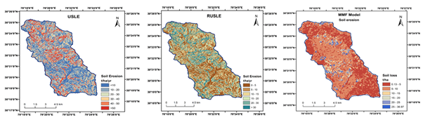
USLE model predicts that about 31% of the watershed area has average annual soil loss in the range of 30-40 t/ha/year while RUSLE model predicts about 35% of the watershed area has erosion rate >30 t/ha/year. Average annual soil loss estimated by the MMF model is found to be comparatively less than the USLE and RUSLE models. Clockwise hysteresis loops for most of the events indicate that sediment supply is mainly from the in-stream channel with limited supply from upland areas.
Soil moisture plays a vital role in the water transport pathway of soil-plant-atmosphere continuum systems. The moisture content of soil is a crucial variable of water and energy cycle as it has a strong influence on energy and water balance. In addition, it determines the proportion of incoming longwave solar radiation into outgoing longwave radiation, latent, sensible, and ground heat flux and partitions the rainfall into the runoff, surface storage, and infiltration components. Soil moisture varies spatially and temporally due to the heterogeneity of soil texture, topography, vegetation and climate and its observations and estimations are complex, time-consuming and expensive. Therefore, an empirical model is developed for estimating soil moisture at different soil depths using readily available meteorological parameters, i.e. rainfall, wind speed, air temperature, and near soil surface temperature and its applicability is checked. The governing equation is given below:

where θt is the soil moisture of present-day, θ(t-1) is the soil moisture of the previous day, P is the precipitation, α and β are coefficients which varies between 0 and 1, U is wind speed at 2 m, µ and λ are coefficients, and ATMax and STMax are the maximum air and soil surface temperature, respectively. From this equation, simplified models corresponding to soil depths of 2 cm, 6 cm, and 25 cm have been derived. A comparison of observed and simulated soil moisture is illustrated in Figure – 6.
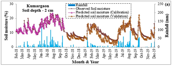
The model performed satisfactorily in calibration and validation for different soil depths. The model is further simplified for field applications tested for its performance. It is found that the simplified model performed well for the topmost layers at the study sites. The model performance decreased with increasing soil depths indicating that the effect of meteorological variables decreases as soil depth increases.